Intro to RNNs | Anirudhh Venkat

The following is a brief history of recurrent networks, discussing RNNs and optimizers. My intention in writing this is to make the basics behind recurrent networks as digestible as possible, however I assume prerequisite knowledge of Calculus 1 and basic machine learning.

Recurrent Neural Networks

We sometimes find ourselves able to predict the next word coming out of someones mouth. For example, if I were to say to you “Let’s go shopping for clothes at the blank,” what would you think comes next?

You would likely guess “mall” because of the words that come prior. If I had asked you to predict what word I’m going to say right now with no knowledge of the words I said before, it would be near impossible.

This is the struggle that feed forward neural networks (FFNs) face . They process inputs independently, meaning in a temporal task, where each input is related to the next, they’re unable to remember information from the previous input.

This is why recurrent neural networks (RNNs) were created; they employ hidden states, which can be thought of as encodings of knowledge associated with a particular layer. RNNs update each layer’s hidden state by multiplying the previous hidden state by a weight matrix, adding the current input times another weight matrix, and then adding a bias term. The weight matrices and bias term are what the network adjusts to control how the previous hidden state and current input affect the current hidden state. $\sigma$ represents an arbitrary activation function, for example ReLU, which will be discussed soon.

$$ \underbrace{h_t}_{\text{Current Hidden State}} = \sigma ( \underbrace{W_{hh} h_{t-1}}_{\text{Previous Hidden State}} + \underbrace{W_{xh} x_t}_{\text{Current Input}} + \underbrace{b_h}_{\text{Bias}} ) $$

The current hidden state is then multiplied by another weight matrix and added to another bias term to form the layer’s output. Similar to before, the weight matrix and bias term are adjusted by the network to control how the current hidden state influences the layer’s output.

$$ \underbrace{y_t}_{\text{Layer Output}} = \sigma_y ( \underbrace{W_{hy} \cdot h_t}_{\text{Current Hidden State}} + \underbrace{b_y}_{\text{Bias}} ) $$

Since the current hidden state $h_t$ is a function of the previous hidden state $h_{t-1}$, and $h_{t-1}$ is a function of the previous input $x_{t-1}$, we can prove by induction that $h_t$ recursively encodes all previous inputs.

Proof by Induction

$\underbrace{h_{1}}_{\text{First Computed State}} = \sigma ( \underbrace{W_{hh} h_{0}}_{\text{Initial Hidden State}} + \underbrace{W_{xh} x_{1}}_{\text{First Input}} + \underbrace{b_h}_{\text{Bias}} )$ $h_1 = f(x_1)$

$$ h_t = f(x_t,x_{t-1},...,x_2,x_1) $$

$$ h_{t+1} = f(x_{t+1},x_{t},x_{t-1}...,x_2,x_1) $$

$$ \underbrace{h_{t+1}}_{\text{Next Hidden State}} = \sigma ( \underbrace{W_{hh} h_{t}}_{\text{Current Hidden State}} + \underbrace{W_{xh} x_{t+1}}_{\text{Next Input}} + \underbrace{b_h}_{\text{Bias}} ) $$

$$ h_{t+1} = \sigma ( W_{hh} f(x_t, x_{t-1}, \dots, x_1) + W_{xh} x_{t+1} + b_h ) $$

Because $f(x_t,x_{t-1},…,x_2,x_1)$ is a function of $x_t,x_{t-1},…,x_2,x_1$, and $x_{t+1}$ is reflexively a function of $x_{t+1}$,

$$ h_{t+1} = f(x_{t+1},x_{t},x_{t-1}...,x_2,x_1) \tag*{$\blacksquare$} $$

This contrasts to FFNs, where the hidden state at timestep $t$ contains a representation of the input $x_t$ only at $t$.

$$ \underbrace{h_t^{(1)}}_{\text{First Layer Output}} = \sigma^{(1)} ( \underbrace{W^{(1)} \cdot x_t}_{\text{Current Input}} + b^{(1)} ) $$

Even though the first layer’s output permeates throughout the network’s layers for each layer $l$, $h_t$ is still only a function of $x_t$.

$\underbrace{h_t^{(l)}}_{\text{Layer Output}} = \sigma^{(l)} ( \underbrace{W^{(l)} \cdot h_t^{(l-1)}}_{\text{Previous Layer Output}} + {b^{(l)}} )$ ${h_t^{(l)}=f(x_t)}$

Backpropagation Throughout Time

As introduced in Rumelhart et al. (1986), standard backpropagation assumes that each layer passes information forwards once. However, in a RNN, information is passed backwards throughout timesteps. So arises the question - how do we apply backpropagation to a RNN?

Werbos (1988) answers this through a process called backpropagation throughout time (BPTT). By creating copies of the network for each timestep, we effectively have $T$ network copies, with $T$ denotes the number of timesteps. Note that the weights for all hidden layers are the same, and likewise for the output layers.

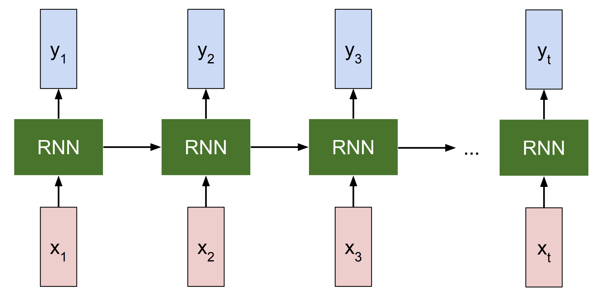
Figure 1. Simplified RNN box (Left) and Unrolled RNN (Right). Adapted from CS231n (n.d.).

Now that we have a network where information is passed forward, we can apply standard backpropagation, but with a twist. Since the weights are the same across timesteps/layers, we need to calculate the summation of the gradients of the loss function wrt to each weight, across all timesteps. Terms $i$ and $j$ represent arbitrary neurons, $w_{ij}$ represents the weight connecting neuron $j$ to neuron $i$, $s_i(t)$ represents the pre activation output of neuron $i$, and $L$ represents the loss function of the network.

$$ \frac{\partial L}{\partial w_{ij}} = \sum_{t=1}^{T} \underbrace{\left( \frac{\partial L}{\partial s_i(t)} \cdot \frac{\partial s_i(t)}{\partial w_{ij}} \right)}_{\text{Chain Rule at step } t} $$

The weight update is calculated by multiplying the summation by the learning rate $a$. The neuron impact ${\frac{\partial L}{\partial s_i(t)}}$ is reflective of how neuron $i$ impacts the loss function $L$, and the weight impact ${\frac{\partial s_i(t)}{\partial w_{ij}}}$ reveals how weight $w_{ij}$ impacts neuron $i$.

$$ \underbrace{\Delta w_{ij}}_{\text{Weight Update}} = - \underbrace{\alpha}_{\text{Learning Rate}} \sum_{t=1}^{T} \left( \underbrace{\frac{\partial L}{\partial s_i(t)}}_{\text{Neuron Impact}} \cdot \underbrace{\frac{\partial s_i(t)}{\partial w_{ij}}}_{\text{Weight Impact}} \right) $$

Its important to note that ${\frac{\partial L}{\partial s_i(t)}}$ is almost always computed via Chain Rule, as the gradient must be computed from neuron $i$’s layer to the output layer. The exception is if neuron $i$ resides in the output layer of the network.

$$ \underbrace{\frac{\partial L}{\partial s_i(t)}}_{\text{Neuron Impact}} = \underbrace{\frac{\partial L}{\partial s_i(T)}}_{\text{Output Neuron Impact}} \cdot \underbrace{\left( \frac{\partial s_i(T)}{\partial s_i(T-1)} \cdot \frac{\partial s_i(T-1)}{\partial s_i(T-2)} \cdot \dots \cdot \frac{\partial s_i(t+1)}{\partial s_i(t)} \right)}_{\text{Sequence of Neuron to Neuron Impacts}} $$

Vanishing/Exploding Gradients

BPTT’s main drawback are vanishing/exploding gradients. If the neuron impact is too small or too large, then $\frac{\partial L}{\partial w_{ij}}$ will either round down to zero or explode to infinity. If the derivatives in the neuron impact sequence are all $<1$, then as $T$ increases, $\frac{\partial L}{\partial s_i(t)}$ comes closer to 0. The opposite holds true as $\frac{\partial L}{\partial s_i(t)}$ comes closer to infinity when the derivatives in the sequence are all $>1$, and $T$ increases. Both outcomes break the learning process.

There are many ways to avoid vanishing/exploding gradients, listed here are just a few:

Figure 2. Residual building block featuring the identity skip connection. Adapted from He et al. (2016).

Real Time Recurrent Learning

Another limitation of BPTT is that it computes all gradients across time steps at once, meaning the network is unable to learn in real time. To truly resemble the human mind, we need a network that can learn on the fly, thus the motivation behind real-time recurrent learning (RTRL) from Williams & Zipser (1989). Unike BPTT which computes gradients after a forward pass, RTRL computes what I like to call “future gradients” during the forward pass, by calculating a sensitivity matrix that determines how changing a weight will impact the output of neurons one timestep in the future.

$$ \underbrace{\frac{\partial y_k(t+1)}{\partial w_{ij}}}_{\text{Next Sensitivity}} = f_k'(s_k(t)) \left[ \underbrace{\sum_{l \in U} w_{kl} \frac{\partial y_l(t)}{\partial w_{ij}}}_{\text{Past Influence}} + \underbrace{\delta_{ik} z_j(t)}_{\text{Current Input}} \right] $$

$$ p_{ij}^k(t) = \frac{\partial y_k(t)}{\partial w_{ij}} $$

Similarly to how the weight update equation in BPTT summates over timesteps $t \in T$, the weight update for RTRL is a summation over neurons $k \in U$.

$$ {\Delta w_{ij}(t)} = \underbrace{\alpha}_{\text{Learning Rate}} \sum_{k \in U} ( \underbrace{e_k(t)}_{\text{Error}} \cdot {p_{ij}^k(t)} ) $$

Comparing the weight update equations for BPTT and RTRL, one can see that their relationship mirrors that of the primal and dual equations used in SVM optimization.

Conclusion

Given the ability to learn online, RTRL seems like it would be better than BPTT right? However RTRL comes with its own set of flaws, the two most prominent being the computational issues that stem from the sensitivity equation. The first is that we need to store $N$ $\cdot$ $W$ values, where $N$ represents the number of neurons in the network, and $W$ the number of weights. Because the network is fully connected, $W$ is $N^2$. The space complexity is therefore $N^3$ = $N$ $\cdot$ $N^2$. The time complexity of RTRL is the second computational issue. Because we need to calculate the sensitivity of each weight $N^2$ to each neuron ($N$), and summate over all neurons ($N$), the time complexity is $N^4$ = $N^2$ $\cdot$ $N$ $\cdot$ $N$.

Another issue is the chance of deviation from global gradient patterns. This is because instead of accumulating gradients across timesteps and then updating (BPTT), we update at each timestep, which is highly sensitive to outliers. A remedy for this is to apply a low learning rate so that no one gradient drastically changes a weight.

These issues make BPTT the standard choice over RTRL. However, if the computational ceiling of RTRL were to be brought down, we would unlock networks that could evolve with every new experience.